Network Analysis: Capabilities of Processing and Transportation

Background and Objectives:

                As a continuation of our semester long Fracture sand mining project, student are asked to evaluate transportation routes using the Network analyst tool in Esri’s ArcMap. As the project moves forward, we prepare data on the significance of impact on the roads from trucking sand to rail terminals. This is a necessary step towards our end goal, because it provides significance and a quantifiable value of the impact on the local infrastructure. The trucking involved with sand mining produces a large effect on local roads because after the process of extracting the sand from the ground it must be transported to a processing facility or fracture mining location for use. For this portion of our project we are looking specifically at the impact on the roads network. To begin to prepare our data for use in the Network Analysis, we must consider the following things:

Which mines will be using trucks only to transport their sand to a rail terminal?

What is the most efficient route to the rail terminal?

How many total miles does each truck drive in individual counties?

What will the cost of the impact on the roads network be for each county?

Procedures: 

Each mine possesses different capabilities of processing and transportation. For example some mines have processing facilities and rail terminals on site, while others, can only transport via truck on roads. In our project, we only concern ourselves with the impact to roads and highways in Wisconsin. To begin, we used python script to help us complete the network analysis. In python, we wrote a script that created shapefiles with pertinent information. This could have been done regularly in ArcMap sessions, but we used this opportunity to further our script writing skills. As displayed in figure 1, the resulting script supplied us with mine locations that are active, are further then 1.5 kilometers from a rail terminal, and don’t have a privately owned rail terminal on location.

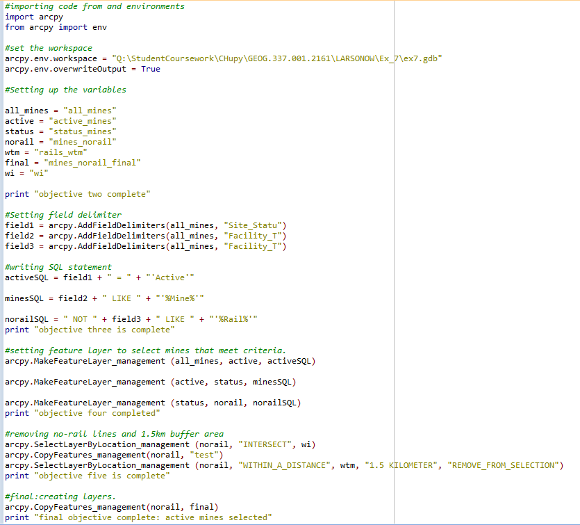
   Figure 1: Python script for running data preparation steps (query) create .shp files for project

                                            

Next I displayed the active mines with no rail terminal in ArcMap. Within the ArcMap software is a native program called Model builder. For simplification of workflow and correct data management we used model builder to use the tools necessary for a completed exercise. After looking at the data in ArcMap, we used Network Analysist, which contains a tool called “Closest Facility”. Closest facility creates a route from incidents (active mines) to the terminal (rail facility) using a street network accessed in ArcMaps. 

Figure 2: Model built for the workflow for the network analysis of fracture sand mining in Wisconsin

This tool allows us to make a line segment out of the route, which in turn supplies us with a number value for the length of road traveled to get the sand to the rail facility. Continuing to build our model, new fields were added on the data table to produce total distance traveled per county, and a cost per county from the road impact. In our hypothetical project, we made up a number for the cost of each mile traveled by road would amount to 2.2 cents. This number is most likely not accurate, but it serves a purpose to help students become familiar with doing cost analysis on transportation routes.

Results: 

Figure 3: State of Wisconsin with counties showing cost in dollars of fracture sand trucking in a gradient of blue. Routes to the closest facilities are displayed in light blue lines from mines (Yellow) to facilities (green).

After the model ran, a final table was produced that contained the total amount of miles driven in each county, and how much hypothetically this would cost. Looking at the distances and cost, it varies quite drastically. This is to be expected as most of the sand available for mining is located in the central portion of west Wisconsin. An important ramification of this project was projects like this have real world consequences. Just recently a group of GIS professionals produced a project with great similarity to ours for the county of Chippewa Falls. The group ran network analysis and risk factors, in much greater detail. As a student this is of great importance for me to gauge how educational projects can be designed with real world implications and geography is a very powerful tool to use.

                Another aspect of this project to consider in discussion is the routes that are taken, and the trueness of the cost calculations. Looking at figure 3, the trucks take their own distinct route, for the most part. For many of the routes, portions of the road driven are not distinctly only one truck route. As trucks come towards a main rail facility they overlap routes. Because we are calculating the cost off distance, this overlap could have a great effect on the overall value of the output. To check to see if the calculations too into effect individual route completely, or it allowed overlap I needed to look at the routes feature class directly. Highlighting routes one by one and looking at the line created I could see if the routes were composed of a true distance, and they were. A final data table shown in figure 4, shows all of the counties that have a cost associated with fracture sand trucking. 

Figure 4: Final table created showing cost and distance traveled in each county by trucks.

The implications of this final table are of vital importance, and could possibly play a role in later decisions for local governments. Figure 4 shows counties like Eau Claire, Chippewa and Barron county incur a great deal of use of roads from sand mining operations. As these number are hypothetical, they hold no inherent value to any governmental body, but the idea behind the information is whats important. Running analysis like this on transportation networks have help save vast amounts of time and money. GIS proves valuable tool or making decisions, and if implemented properly can gain many meaningful insights to operations that may not have normally been obvious. 

Conclusions: A formal report of findings is required to discuss findings. Throughout the process of this project, students are learning "best practices" for GIS programs. Structuring decisions based off data integrity and aiming for meaningful answers push students to be thoughtful in how they compose their analysis. Using programs like Model Builder and Python allow students to simplify workflow and naming structure in a way that facilitates more composed answers. Outlining the perimeters of the project allow for transparency with data analysis. This particular exercise utilized Network Analysis tools to route trucks to a closest facility for rail transportation. This tool allowed us to calculate a rough hypothesis of the cost individual counties experience from trucking fracture sand. The implications of this information could impact decisions on local infrastructure spending, taxes, and traffic flow. As a training GIS analyist, projects like this, which have real-world counter parts are a great practice for possible career projects later in life. 

Geocoding; Normalized Address Tables

Objectives: As part of the technical report following the Geocoding and Table Normalization portion of our fracture sand mining project, a few overarching objectives were outlined to give students clear understanding of the techniques and skills involved in Geocoding using a GIS program. For this project, we were supplied with a data table of the facture sand mines located in Wisconsin from the Department of Natural Resources (DNR). Presented with this table of facility and locational information, we needed to organize the structure of rows and columns into separated address attributes to allow for efficient loading in the correct manner into the Esri program ArcMap. The activity of organizing is called table normalization and is a critical part to begin to locate the mines via geocoding. By separating out the address and PPLS information we allow Esri software to place the mine location on the map more accurately. Along with geocoding, Table normalization will prove to be a valuable tool as this project moves forward.

Methods:  The next portion to build towards the overall project goal is to process the mine locations with the end result of geocoded mines in the correct location.To begin, the normalized table is loaded into Esri ArcMap, followed by loading a base map which to aid in location the mines along with PPLS quarter sections. As the geocoding tool bar is activated, Esri automatically matches the mine attribute to a location on the map based on ether the local street address or PPLS address. The automatic matching is often not every accurate, especially when only the PPLS address is given as Esri's system doesn't function with PPLS information. Concerns with accuracy of automated matching will be addressed upon completion of the project. Once all the mines are plotted students went through the strenuous and sometimes confusing task of negotiating if the mine is actually located in the spot, or not. Students have a tool box of ways to accomplish this, some of which include a GoogleMaps search, using a Ersi Base map, or even a PPLS finder online if the mine is particularly hard to locate. Once the most accurate approximation of the location is made, the student manually matches the mine to the location using the Geocoder toolbar. For each mine the steps are repeated. However the great variety of address information made the task more of a challenge. Some of the mine information did not contain a street address or only possessed a PPLS address. This did provide an added element of complexity, but nothing that time and diligence could not overcome. After all the mines have been geocoded, the objective is to move to a dataset of high accuracy and check your geocoded locations against the actually mine locations.

Results:

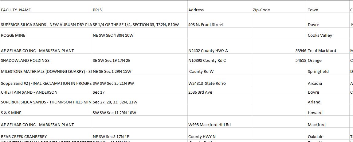
 Pictured to the right is an example of ordinary address data. The table contains information about street and PPLS information in the same column, along with several other types of information contains in each cell.

  By dividing the various elements of each mine into its own unique field, the information could be used to geocode the location of the mines. The resulting Table below has been appropriately normalized. 

 Figure 1: Non-Normalized table contains 

multiple pieces of attribute information in each cell.  

  By dividing the various elements of each mine

 into its own unique field, the information could be 
used to geocode the location of the mines. 
The resulting Table below has been appropriately normalized. 

Figure 2: This table has been normalized in such a manner that allows for efficient loading into Ersi ArcMaps. Each column contains one type of information. A normalized table contains individual attributes separately to maximize clarity of address. 

              



                           A few of the mines only contain a street address, while others have only a PPLS address. These types of inconsistencies make it hard to automatically plot all of the mines accurately. Steps must be taken by the individual to facilitate accurate geocoding. Tools like Google Maps, and online PPLS locators can aid in locating the mine if the individual is not able to find the mine in ArcMap using a PPLS address feature class.
                         After time has been taken to individually place each location of the mine to the best ability, the mine actual locations are imported into ArcMap after being obtained from a facility member of the University. It is always best practices to test for accuracy using a dataset with a higher degree of accuracy then the data set you are working with. To analyze how closely my geocoded mine locations  matched the closeness of coordinate data of the true positions of the real world feature mines, I used a native Ersi data management tool "Near". 

Figure 3: Locations of assigned mines vs true locations of mines.
Base map source: Esri Online 2013 Esri.com

This tool located the mine with the corresponding unique Mine_ID which each mine feature class contains. The Near tool created a new feature class as a result of the analysis in the source table, which was my mapped/geocoded mines. The new field contains the closeness of my geocoded mine to the true mine locations. Figure 3 shows mines locations in green and yellow, my mines being the former, and the true locations the latter. 

         Figure 4 below is the attribute table after I ran the near tool. The highlighted field shows the distances in meters of the mines. Some were placed quite close the true locations, while others missed altogether, as is the case of the last two mines. Although the accuracy was not very stellar for the set as a whole, lessons learned are very important. Computer programs often require getting "dirty" with the data, using and manipulating while aiming to learn best practices requires time and experience. This dataset provided great experienced in the class to help gear students work in real world situations and data.

Figure 4: Fields in source table (my mapped mines), highlighted in blue is the distance field
 on how closely my mines matched the true mines.

Data Collection and Project Overview

                Goals and Objectives:

In the Context of this lab project for Geography 337, students will be learning how to properly download and use data gathered from several online platforms by a variety of organizations. The purpose of learning proper data management is to make sure students are comfortable with seeing and using multiple different data formats and download platforms. Previous to this lab, students have been given “canned” data from Esri services which is already perfectly organized and groomed for easy use in assignments. In the real world of data, clean and perfectly groomed data is never a sure thing. In order to prepare for future jobs this project aims to further familiarize students with proper techniques in downloading and using data in a geographic context of mining in Wisconsin for sand used primarily in hydrofracture mining conducted across the country for natural gas and oil used to produce energy.

General Methods Used:

                To get started with this semester long project, students first needed to obtain data from different sources online. Our first stop for information was the US Department of Transportation to get NTAD data on the railway network. The online downloading platform for this site was easy to manage and provided quality metadata for the datasets used. The next stop was to compile data for land cover, for this we went to the USGS National map viewer. The map viewer allowed access to a great abundance of different types of information about ground cover across the United States. Specifically we are only interested in the NLCD (National Ground Cover Data) for Tremealeau Co, WI.

                The third stop for data collection in this project is to the USDA, which has a simple Data Gateways platform for downloading data. Here we downloaded the Crop land data layer as well as the metadata for the set which we downloaded. The next step in data acquisition was the Trempealeau County database and land records. This county data base has a bunch of great information we will find useful over the projects duration, because of this we will download the entire database.

                The final data collection step we needed to accomplish was gathering Soil data, which can be done from the USDA NRCS web soil survey (WSS). This dataset was the trickiest to navigate and required more time to get the data into a useable format for our project. After we downloaded the SSURGO data from the WSS, we performed a join and relationship class to get the current soil information into the TMP (Trempealeau, Co.) geo database we downloaded.

Now that we have all the Data in the right place on our computers, we unzipped the files into a working folder. The unzipped files were then looked at, and important features were extracted, in particular the Raster’s for land cover and crop land cover. Now our data acquisition is complete, and can begin the next portion of the project, which is to write a Python script to project and clip/extract by mask the raster’s and load them into our geodatabase.

Figure 1: Displays the three raster's which we downloaded from online platforms. A. displays the Landcover (USGS 2013), B. displays the Crop land cover (USDA 2011), C. displays the  elevation model (DEM) from USGS. D. is a locator map for Trempealeau Co, WI.

Data Accuracy:

 As part of downloading data, reviewing pertinent metadata is very important. Accuracy standards hold great consequence for projects in the real world. After the data was collected, we looked inside each metadata set and compiled a chart of how accurate the data is and other important lineage information. This documentation is important for credibility and how confident you can be in the final project to contain real-world truth, and be of use for the application. 

Figure 2: A table of various accuracy information from the metadata compiled from the online sources. 

Python Script

Python script is a native computer code which can be used to run tools and set perimeters inside of Esri's ArcMap program. Python code can be very useful in performing tasks because it is a language which facilitates batch-processing and allows users to process multiple data set simultaneously.Furthermore Python coding also helps organize and keep track of data information prior to the mapping process which streamlines product completion. The Python scripts follow proper formatting protocol which help enable users to perform "Best Practices", and also allows users to further data integrity when using analysis tools.

In this first excersize, we were introduced to python coding, and used it to facilitate the projection, extraction(load) and clip 3 rasters which we downloaded from online sources. For our project, this enabled us to quickly and efficiently work with our raster data sets. Python is very expansive and powerful, and can be used by a variety of computer programs.

Python Code One:

Figure 1: Python coding used to project, extract and clip multiple raster datasets in our Sandmineing project.

Figure 2: Displaying the python code written for exercise 7. The script loads and projects rasters in a Batch format. Delineation and setting variables facilitated a efficient system for the sand mine project.

Blog Post 1

Hydro Fracturing in Western Wisconsin: An Overview

Wisconsin and Fracture Sand: A Brief Introduction

Today, energy consumption in the United States is at an all time high, with no signs of slowing down anytime soon. Because of this national influence, states like Wisconsin has been put in a special situation. In order to increase domestic production of energy (mainly oil and natural gas), companies across the country have been increasing hydrolic fracturing operations. Hydrolic facturing requires a very specific type of quartz sand which can be used during the fracturing process. Wisconsin contains the greatest deposits of this quartz sand in the United States, and because of this has become a sand mining hot spot. 

Implications: In a variety of ways, frac-sand has become a much debated topic. From economic consequences, to environmental concerns, frac-sand is an important issue. Focusing only on how the sand mining influences the state, several issues can be discussed directly. Firstly, how the sand mining in western Wisconsin effects the local residents (health, and economic functions). Secondly, how the sand mining is transported out of the state to the operational sites where the holes are drilled and gas produced. 

For the purposes of this lab, we will analyze frac-sand efficiency in transportation and mine operations using Esri ArcGIS programs with information provided by the State DNR, and national data from NCRS soil survey, USDS and USDA. The purpose of this blog post specifically is to give background information on the mining operations and the logistics behind the fracturing process. 

Hydrolic Frac-Sand Mining

For decades, hydrolic fracture mining has been a technique used to extract natural gas and oil from deep within the earth surface for industrial, commercial, and residential energy production. Hydrolic-fracturing consists of drilling kilometers down into the earths crust, typically into the layer of shale rock which holds the natural gas and oil, pumping silica sand (Frac-sand for short), water and various chemicals into the hole. After the water and sand has been pumped in at great pressure, the rock fractures releasing the desired gas or oil which is normally trapped by the weight of the rocks pressing down.
This is a simplistic explanation of the highly technical process involved, called horizontal hydrolic fracturing, displayed below:

Figure 1: Horizontal fracturing technique

(http://www.enviromineinc.com/got-frac-sand/)

Silica Sand (Quartz)

Quartz sand is practically suited for use in hydrolic fracturing processes because of its perfectly rounded size, extreme pressure capabilities and uniformity in size. Once the sand is pumped into the the drilled hole, the rounded size props open the small fissures created by the pressure of the water. The water is then pumped out leaving the sand behind keeping the fissures open. If the sand could not withstand such great pressure, the cracks would close leaving the gas or oil unobtainable. 

Quartz sand is also particularly easy to mine, requiring only minimal hole creation and post-mining processes to obtain the completed product.

Figure 2: close up image of silica sand holding a crack open

(www.jasonmunster.com)

Where can the Sand be found?

Wisconsin is located in such a region that contains great deposits of silica sand. This is mainly because the Sands that meet these specifications are mined from poorly cemented Cambrian and Ordovician sandstone's which are abundant in western Wisconsin which were previously marine coastlines during the late Cambrian period. Another advantage of the location of the sand in Wisconsin is that during the periods of glaciation the part of western Wisconsin were left untouched by glaciers leaving the uniform size of the sand intact. 

Figure 3: locations in Wisconsin of Quartz sand 

(http://www.isthmus.com/media/2014/03/20/586CoverIndustrialSandPotential3912.jpg)

Primary regions of Natural gas production

Figure 4: Map of United States showing Natural gas (in red)

(Wisconsin DNR)

Overview of GIS in project

Primarily Geospatial information system can be used to implement efficient and effective routes to direct the traffic of trucks from the mine to a particular rail station for further transport across the country to specific fracturing sites. Another application of GIS programs is operational productivity of the mines. Monitering the volume of sand produced each day or month can be done in a GIS program and be used to ensure peak productivity of the mine and the workers. As we all know time is money, so being efficient and productive to the greatest extent is key to a profitable mining operation. 

Sources:

West Central Wisconsin Regional Planning Commission

http://wcwrpc.org/frac-sand-factsheet.pdf (accessed 10.20.15)

Wisconsin Department of Natural Resources

http://dnr.wi.gov/topic/Mines/documents/SilicaSandMiningFinal.pdf (accessed 10.19.15)

Isthmus Online Newspaper

http://www.isthmus.com/media/2014/03/20/586CoverIndustrialSandPotential3912.jpg

Image of Quartz Sand:

www.jasonmunster.com (Accessed 10.20.15)

http://www.wintershall.com/

Image of Hydro fracturing Diagram

http://www.enviromineinc.com/got-frac-sand/ (Accessed 10.20.15)

(Courtesy of First Electric Newspaper (2012))